|
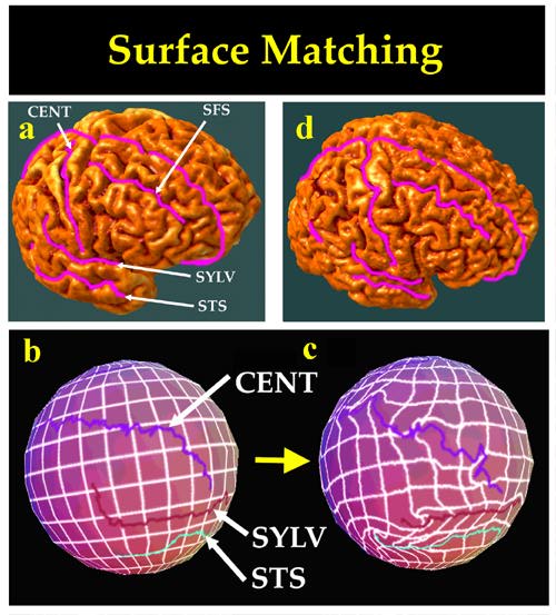
| Fig. 8. Scheme to Match Cortical Regions with High-Dimensional Transformations and Color-Coded Spherical Maps. |
by
Paul Thompson
III. Cortical Surface Matching
Cortical patterns are so complex that specialized algorithms are needed to match them. Cortical surfaces can be matched using a procedure which also matches large networks of gyral and sulcal landmarks with their counterparts in the target brain (Drury et al., 1996; Davatzikos, 1996; Thompson and Toga, 1996, 1997; Van Essen et al., 1997). Differences in the serial organization of cortical gyri prevent exact gyrus-by-gyrus matching of one cortex with another, but an important intermediate goal has been to match a comprehensive network of sulcal and gyral elements which are consistent in their incidence and topology across subjects. Elastic matching of primary cortical regions factors out a substantial component of confounding cortical variance in functional imaging studies, as it directly compensates for drastic variations in cortical patterns across subjects (Steinmetz et al., 1990; Woods, 1996; Thompson et al., 1997). Quantitative comparison of cortical models can also be based on the mapping which drives one cortex with another (Van Essen et al., 1997; Thompson et al., 1997). Because of its role in our pathology detection algorithm discussed later (Section 4), we will focus on this mapping procedure in some detail.
Summary of Method. Our method (Thompson and Toga, 1996) is conceptually similar to that of (Davatzikos, 1996). 3D active surfaces (Cohen and Cohen, 1992) are used to automatically extract parametric representations of each subject's cortex, on which corresponding networks of anatomical curves are identified. The transformation relating these networks is expressed as a vector flow field in the parameter space of the cortex (Fig. 8). This vector flow field in parameter space indirectly specifies a correspondence field in 3D, which drives one cortical surface into the shape of another. This mapping matches up every element of the specified system of landmark curves with its counterpart in the target brain.
|
|
| Fig. 8. Scheme to Match Cortical Regions with High-Dimensional Transformations and Color-Coded Spherical Maps. |
Algorithm Details. Several algorithms have been proposed to extract cortical surface models from 3D MR data (Sandor and Leahy, 1995; Davatzikos and Prince, 1996; Xu and Prince, 1996; Davatzikos, 1996). In one algorithm (MacDonald et al., 1993), a spherical mesh surface is continuously deformed to match a target boundary defined by a threshold value in the continuous 3D MR image intensity field. Evolution of the deformable surface is constrained by systems of partial differential equations. These equations have terms that attract the parametric model to regions with the pre-selected intensity value, while penalizing excessive local bending or stretching (but see Footnote 3). If an initial estimate of the surface v0(s,r) is provided as a boundary condition (see Thompson and Toga, 1996, for details), the final position of the surface is given by the solution (as t tends to infinity) of the Euler-Lagrange evolution equation:
dv/dt -d/ds(w10|dv/ds|)-d/dr(w01|dv/dr|)+2d2/dsdr(w11|d2v/dsdr|)
+d2/ds2(w20 |d2v/ds2|)+d2/dr2(w02|d2v/dr2|) = F(v).
Here F(v) is the sum of the external forces applied to the surface, d/ds and d/dr represent partial derivatives with respect to s and r, and the wij terms improve the regularity of the surface. The spherical parameterization of the deforming surface is maintained under the complex transformation, and the resulting model of the cortex consists of a high-resolution mesh of discrete triangular elements that tile the surface.
Footnote 3
. Deformable surface models often have difficulty in extracting surfaces of structures with extremely complex geometry, such as the ventricles and caudate, due to their irregular or 3D spiral nature, and modifying their behavior is the topic of active research (Cohen and Cohen, 1992; Davatzikos and Prince, 1996; Xu and Prince, 1996). Interestingly, many 3D image warping algorithms are capable of diffeomorphically transforming an irregular or spiral structure into a more regular shape. This more regular shape can then be used as the target for automated surface extraction. The resulting regular surface model can then be back-transformed (using the inverse of the transformation used to warp the underlying image) to reflect its actual irregular geometry. Alternatively, by applying the inverse of the derived 3D deformation field to a regular 3D lattice ruled over the warped 3D image, a reparameterization of the original image with a 3D curvilinear computational mesh is obtained. Since the Riemannian metric tensor of this reparameterization is known, the PDE governing surface extraction can be rewritten in covariant notation (see later, Section 3) and run directly on the original image, using accessory 3D arrays of Christoffel symbols and metric tensor coefficients, obtained from the 3D warping algorithm, to correct the forms of the differential operators. We are currently testing this locally-adaptive modification of the core surface extraction algorithm. In particular, the solution of the surface extraction equation on a 3D curvilinear mesh biases the dynamics of the deforming surface in favor of the expected geometry of the surface to be extracted, without the need to resample the image in which the surface evolves.Colorized RGB maps of the Cortical Parameter Space. Because the cortical model is arrived at by the deformation of a spherical mesh, any point on the cortical surface (Fig. 8(a)) must map to exactly one point on the sphere (Fig. 8(b)), and vice versa. Each cortical surface is parameterized with an invertible mapping Dp,Dq: (r,s)-> (x,y,z), so sulcal curves and landmarks in the folded brain surface can be reidentified in the spherical map (cf. Sereno et al., 1996 for a similar approach; see also Footnote 4 and Fig. 8(b)). To retain relevant 3D information, cortical surface point position vectors in 3D stereotaxic space are color-coded at 16 bits per channel, to form an image of the parameter space in RGB color image format [Fig. 8(b)/(c)]. To find good matches between cortical regions in different subjects [Fig. 8(a)/(d)], we first derive a spherical map for each respective surface model [Fig. 8(b)/(c)] and then perform the matching process in the spherical parametric space, W . The parameter shift function u(r):W -> W , is given by the solution Fpq:r->r+u(r) to a curve-driven warp in the biperiodic parametric space W =[0,2.pi)x[0,pi) of the external cortex (Fig. 9; cf. Davatzikos, 1996; Drury et al., 1996a; Van Essen et al., 1997).

|
| Fig. 9. Matching Gyral Patterns from One Subject to Another, to Measure Cortical Variability. |
Footnote 4: Color-coded spherical maps store geometric and topological information about the sulcal pattern in a 2D array structure which simplifies feature localization and comparison. Cortical models can also be flattened into a fully 2D planar representation (Van Essen and Maunsell, 1990; Schwartz and Merker, 1986; Carman et al., 1995; Drury et al., 1996; Van Essen et al., 1997). Here, the challenging issue of creating planar 2D maps which optimally preserve point-to-point distances is avoided, because the 16-bit color-encoding of the spherical map enables measures of in-surface distance between points on the cortex to computed from the 3D cortical model directly, rather than from a derived or flattened map of the cortical parameter space.
Cortical Curvature. At first sight it seems that the previous approach, using ordinary differential operators to constrain the mapping, can be applied directly. For points r=(r,s) in the parameter space, a system of simultaneous partial differential equations can be written for u(r) using:
L(u(r)) + F(r-u(r)) = 0, for all r in W ,
u(r) = u0(r) , for all r in M0 or M1.
Here M0, M1 are sets of points and (sulcal and gyral) curves where vectors u(r) = u0(r) matching regions of one anatomy with their counterparts in the other are known, and L and F are 2-dimensional equivalents of the differential operators and body forces defined above. Unfortunately, the recovered solution x->Dq(Fpq(Dp-1(x))) will in general be prone to variations in the metric tensors gjk(rp) and gjk(rq) of the mappings Dp and Dq. Since the cortex is not a developable surface (Davatzikos, 1996), it cannot be given a parameterization whose metric tensor is uniform (see Footnote 5). As in fluid dynamics or general relativity applications, the intrinsic curvature of the solution domain should be taken into account when computing flow vector fields in the cortical parameter space, and mapping one mesh surface onto another.
Footnote 5. A tensor-based model of the cortex was introduced for biometric applications in a theoretical paper by Bookstein (Bookstein, 1995). In (Thompson and Toga, 1998), we introduce a covariant formalism as a means to directly incorporate metric tensor information into the regularization equations governing the cortical matching process.
Covariant Formalism. To counteract this problem, we developed a covariant formalism (Thompson and Toga, 1998) which makes cortical mappings independent of how each cortical model is parameterized. This mathematical strategy was introduced by Einstein (1914) to allow the solution of physical field equations defined by elliptic operators on manifolds with intrinsic curvature. Similarly, the problem of deforming one cortex onto another involves solving a similar system of elliptic partial differential equations (Drury et al., 1996; Davatzikos, 1996; Thompson and Toga, 1998), defined on an intrinsically curved computational mesh (in the shape of the cortex). In the covariant formalism, the forms of the differential operators governing the mapping of one cortex to another are modified in an adaptive way which reflects the changes in the underlying metric tensor of the surface parameterizations.
Summary of Covariant Approach to Cortical Matching. Cortical surfaces are matched as follows. We first establish the cortical parameterization, in each subject, as the solution of a time-dependent partial differential equation (PDE) with a spherical computational mesh (Thompson and Toga, 1996; Davatzikos, 1996). This procedure sets up an invertible parameterization of each surface in deformable spherical coordinates (Fig. 9), and allows direct computation of the metric tensors gjk(rp) and gjk(rq) of the mappings. The solution to this PDE defines a Riemannian manifold (Bookstein, 1995). In contrast to prior approaches, this Riemannian manifold is then not flattened (as in Drury et al., 1996; Van Essen et al., 1997), but is used directly as a computational mesh on which a second PDE is defined (see Fig. 10). The second PDE matches sulcal networks from subject to subject. Dependencies between the metric tensors of the underlying surface parameterizations and the matching field itself are eliminated through the use of generalized coordinates and Christoffel symbols (Thompson and Toga, 1998). In the PDE formulation, we replace L by the covariant differential operator L#. In L#, all L's partial derivatives are replaced with covariant derivatives. These covariant derivatives are defined with respect to the metric tensor of the surface domain where calculations are performed.

|
| Fig. 10. Covariant Tensor Approach to Cortical Matching. |
The covariant derivative of a (contravariant) vector field, ui(x), is defined as (Schutz, 1990):
ui,k = duj/dxk + G jik ui (20)
where d represents partial derivative, and the G jik are Christoffel symbols of the second kind. This expression involves not only the rate of change of the vector field itself, as we move along the cortical model, but also the rate of change of the local basis, which itself varies due to the intrinsic curvature of the cortex (cf. Joshi et al., 1995b). On a surface with no intrinsic curvature, the extra terms (Christoffel symbols) vanish. The Christoffel symbols are expressed in terms of derivatives of components of the metric tensor gjk(x), which can be calculated directly from the cortical model:
G ijk = (1/2) gil (dglj/dxk+dglk/dxj-dgjk/dxi ). (21)
Scalar, vector and tensor quantities, in addition to the Christoffel symbols required to implement the diffusion operators on a curved manifold are evaluated by finite differences. These correction terms are then used in the solution of the Dirichlet problem for matching one cortex with another (see Footnote 6).
Footnote 6. Several factors complicate the direct application of covariant regularization equations to cortical anatomic data. In fluid mechanics and general relativity applications, usually a single metric tensor field relates the computation mesh to the physical domain of the data, and the solution to the problem is then back-transformed from the computational mesh to the physical domain. In this application however, different metric tensors gjk(rp) and gjk(rq) relate (1) the physical domain of the input data to the computation mesh (via mapping Dp-1), and (2) the solution on the computation mesh to the output data domain (via mapping Dq). To address this problem (Fig. 10), the PDE L##u(rq)=-F is solved first, to find a flow field Tq:r->r-u(r) on the target spherical map with anatomically-driven boundary conditions u(rq) = u0(rq), for all rq in M0 or M1. Here L## is the covariant adjustment of the differential operator L with respect to the tensor field gjk(rq) induced by Dq. Next, the PDE L#u(rp)=-F is solved, to find a reparameterization Tp:r->r-u(r) of the initial spherical map with boundary conditions u(rp) = 0, for all rp in M0 or M1. Here L# is the covariant adjustment of L with respect to the tensor field gjk(rp) induced by Dp. The full cortical matching field (Fig. 9) is then defined as x->Dq(Fpq(Dp-1(x))) with Fpq = (Tq) -1o (Tp) -1.
Advantages. Using this method, surface matching can be driven by anatomically significant surface features, and the mappings are independent of the chosen parameterization for the surfaces being matched. High spatial accuracy of the match is guaranteed in regions of functional significance or structural complexity, such as sulcal curves and cortical landmarks (Fig. 8). Consequently, the transformation of one cortical surface model onto another is parameterized by one translation vector for each mesh point in the surface model, or 3x65536 ~ 0.2 million parameters. This high-dimensional parameterization of the transformation is required to accommodate fine anatomical variations (cf. Christensen et al., 1995).
This concludes our discussion of warping algorithms. Next, we see how warping algorithms can be used as image analysis tools to support pathology detection in individual subjects or groups.
(to be continued...)Paul Thompson
| RESUME| E-MAIL ME| PERSONAL HOMEPAGE| PROJECTS |
|---|