Computational Anatomy Tools

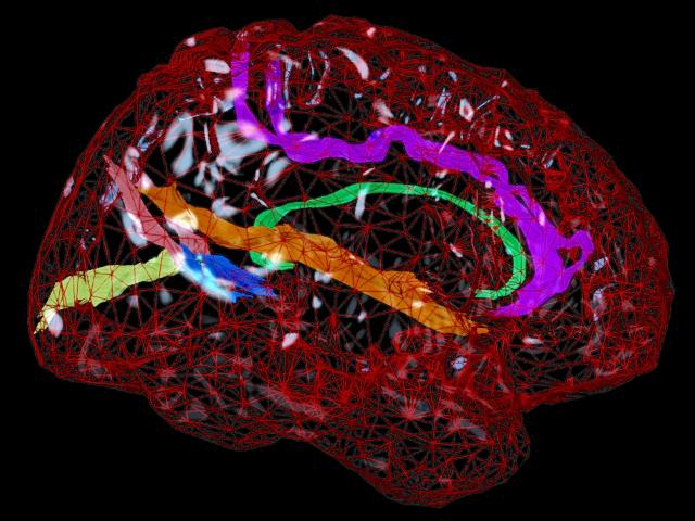
Mesh Models of Anatomy. For many years we have been developing software for computational anatomy. This software allows researchers to build and analyze 3D computational models of anatomical structures. These models can be compared and averaged across subjects, to identify systematic differences in brain structure, and to reveal how the brain varies across subjects, across age, by gender, and in different disease processes. The relationship between brain structure and cognitive, clinical, genetic, and therapeutic parameters can be determined. Patterns of pathology can be identified in an individual or a patient group. Brain changes in response to therapy can also be mapped. By assembling large databases of anatomical models across subjects, striking patterns of anatomy emerge that are not apparent in individual subjects. We use these models to investigate the major diseases of the human brain, including Alzheimer's Disease, schizophrenia, brain tumors, as well as normal and abnormal brain development. Accurate detection and encoding of anatomic differences between subjects often requires mathematical tools that store measures of anatomical variability in normal subjects and use this information to map patterns of abnormal anatomy in new subjects.

Documentation (for internal use):

Contents:

1. Directory Locations of Code

Measuring Manually Traced Surfaces (UCFs):

2. Making Meshes
3. Averaging Meshes; Making Variability, Asymmetry and Displacement Maps
4. Geometric Operations on a UCF (reflecting/reordering)
5. Joining and Splitting UCFs (e.g. partitioning the callosum)
6. Measuring UCFs

Cortical Surface Analyses:

7. Creating and Warping Cortical Flat Maps
8. Medial Cortex Models
9. Mapping Gray Matter Distribution
10. Mapping Cortical Thickness
11. Analyzing Cortical Complexity
Analyzing Surface Maps (4D UCFs):
12. Permutation Tests - for Statistical Effects on Surfaces
Permutation Tests - with Small Volume Corrections
Permutation Tests - Separating Positive and Negative Effects
Permutation Tests - Multi-thresholding
13. Multivariate Regression on Surface Maps
i. Quadratic Regression
ii. Multiple Regression
14. Longitudinal Maps (Rates of Change)
15. T Tests for 4D Maps (Rates of Change, Asymmetry; one-sample, paired samples, permutations)
16. 3D Elastic Warping
17. Format Converters

Directory Locations of Code are shown for each Program (these paths should be added to your .cshrc $PATH variable or specified in your shell scripts):

$SGI means /data/ad/mass3/users/PAULS_SURFACE_CODE/SGI/
$FIX means /data/ad/mass3/users/PAULS_SURFACE_CODE/SGI/FIX/
$4D_UCFS means /data/ad/mass3/users/PAULS_SURFACE_CODE/SGI/4D_UCFS/
$GRAY2 means /data/ad/mass3/users/PAULS_SURFACE_CODE/SGI/4D_UCFS/GRAY2/
$EC means /data/ad/mass3/users/PAULS_SURFACE_CODE/SGI/4D_UCFS/GRAY2/EAT_CLAMPED/
$ARB means /data/ad/mass3/users/PAULS_SURFACE_CODE/SGI/4D_UCFS/ARB/
$ROI means /data/ad/mass3/users/PAULS_SURFACE_CODE/SGI/4D_UCFS/ARB/ROI/
$T_MAPS means /data/ad/mass3/users/PAULS_SURFACE_CODE/SGI/4D_UCFS/ARB/T_MAPS/
$TSGI means /nethome/users/thompson/SGI/
$ASYM means /nethome/users/thompson/SGI/ASYM/
$AFIX means /nethome/users/thompson/SGI/ASYM/FIX/
$JOIN means /nethome/users/thompson/SGI/MESH_JOIN/
$AMIR means /nethome/users/thompson/AMIR_CODE/
$HIPPO means /nethome/users/thompson/HIPPO/SGI/
$COMP means /nethome/users/thompson/COMPLEXITY/
$SEGSGI means /nethome/users/thompson/SEG/SGI/
$WSGI means /data/warp/VARMAP/SGI/
$UM means /data/ad/mass3/users/PAULS_SURFACE_CODE/SGI/MINC/UCF4D_TO_MINC/
$AD means /data/ad/mass2/9p_atlas/CODE/
$XI means /data/warp/paul/ANNOYING/XIAOBO/
$SFLD means /data/ad/mass3/users/PAULS_SURFACE_CODE/SGI/MINC/SFLD_RESAMPLE_MINC/
$EW means /data/ad/mass3/users/PAULS_SURFACE_CODE/SGI/MINC/E_WARP_IMG/ $HEM_FLAT means /nethome/users/thompson/HEM_FLAT/
$MULTREG means /nethome/users/thompson/MULTREG/
$ISO means /nethome/users/thompson/ISOLATED/
$ISOM means /nethome/users/thompson/ISOLATED/MINC/

Making Meshes (programs in $FIX):

redigarb Smooths a surface. Converts a UCF (made with 'seg') into a UCF with 100 uniformly spaced points per level (an RS*.ucf file); assumes Z values are constant within each level (true if input is made with 'seg')
reslicer Makes a parametric mesh. Converts, by redigitizing, an RS*.ucf file (made with redigarb) into a UCF with 150 uniformly spaced levels and 100 uniformly spaced points per level (a parametric mesh, or RSP*.ucf file)
ucf_to_mesh Used less often. Combines the above two operations and makes a mesh directly from a UCF drawn in 'seg'. [In $SGI].

Making a Mesh. Q. How do I make a Mesh from a UCF I have traced?. A. Suppose you traced my.ucf, you use:

/data/ad/mass3/users/PAULS_SURFACE_CODE/SGI/FIX/redigarb 1 2 3 4 5 6 my.ucf > uniform_points_my.ucf
/data/ad/mass3/users/PAULS_SURFACE_CODE/SGI/FIX/reslicer 1 2 3 4 5 6 uniform_points_my.ucf > uniform_slicing_my.ucf

if you want to check how they look, view them (on autarch) with:

~thompson/vu uniform_points_my.ucf
~thompson/vu uniform_slicing_my.ucf

redig_hi Used rarely. Redigitizes a UCF at 1000 points per level, to avoid loss of cross-sectional area if the UCF is subsequently partitioned. See partitioning of the corpus callosum, below. [In $AMIR].

Averaging Meshes; Making Variability, Asymmetry and Displacement Maps (programs in $SGI):

3D_redigarb Same as redigarb, but Z values need not be constant within each level.
3D_reslicer Same as reslicer, but Z values need not be constant within each level.
two_surf_dist Measures 3D distance between two parametric meshes. Outputs a 4D UCF, where the 4th parameter is the displacement between pairs of corresponding points on the two surfaces.
two_surf_dist_XY Measures 3D distance between two parametric meshes, but ignores differences in the Z-direction (this is usually left-to-right in the brain). Outputs a 4D UCF, where the 4th parameter is the displacement between pairs of corresponding points on the two surfaces. Useful in mapping asymmetry, to factor out differences in lateral position, or width, of each structure. [In $ASYM]
arb_two_surf_dist Same as two_surf_dist, but works on cortical surfaces, which have an arbitrary (arb; or spherical) parameterization. [In $ASYM/FIX].
arb_two_surf_dist_XY Same as two_surf_dist_XY, but works on cortical surfaces, which have an arbitrary (arb; or spherical) parameterization. Used to map cortical asymmetry. [In $ASYM].
arb_two_surf_dist_YZ Same as arb_two_surf_dist_XY, but projects out differences along the X direction (this is lateral in ICBM standard space). Used to map cortical asymmetry. [In $AFIX].

Note on Mapping Asymmetry or Displacement in One Plane, or One Direction, only. There is also some code that computes asymmetry along the Y axis only or along Z only. It will compute differences in the cortical pattern to reveal whether a structure is shifted anteriorly (Y) or elevated (Z) relative to its counterpart in the other hemisphere.

You apply it, like the other code, to a UCF line and a flipped (in X) version of its counterpart from the other hemisphere. Note you will see numbers that reflect the coordinate of the second file minus the first; positive values mean the second (flipped) file is higher than the first, or farther forward than the first; negative values mean the second (flipped) file is lower than the first, further back. The value it gives for the bottom point will be exactly the same as the values you graphed for the difference between the Y-min of one side and the other.

EXAMPLE:
You should be able to just replace YZ in the script with Y or with Z:

~thompson/SEG/SGI/two_surf_dist_Y 1 2 3 4 5 6 01L.ucf Xflip_01R.ucf 1L.ucf Xflip_01R.ucf 1L.ucf Xflip_01R.ucf 1L.ucf > asym_along_Y_01.ucf
~thompson/SEG/SGI/two_surf_dist_Z 1 2 3 4 5 6 01L.ucf Xflip_01R.ucf 1L.ucf Xflip_01R.ucf 1L.ucf Xflip_01R.ucf 1L.ucf > asym_along_Z_01.ucf

NOTE
1 2 3 4 5 6 are just dummy variables, values are not used here 7 filenames, only 1st and 2nd are used; values are output on the 7th file, in theory you might want to plot the results on an individual, I just used the 1st (unflipped) surface again.

Note on Parameterizations of Meshes. 'arb' (arbitrary) is just the name for the way the cortex models are parameterized. It means all models are the same (point count per level, level count, and order) but the exact point count per level, level count are arbitrary (anything). This contrasts with some earlier code for surface mesh or surface line averaging, which assumes meshes are 100 points x150 levels ('RSP' files).

Note on Mapping Brain Asymmetry.
The main code for making maps of brain asymmetry is in:
~thompson/SGI/ASYM/FIX/arb_two_surf_dist_YZ
Note some of the asymmetry scripts are set up to work on a coordinate system in which Z is left-right, but you will be fine if you use this 'YZ' code and flip in X.

2. Some scripts that might help in running the asymmetry maps are in here:
cd /data/ad/scratch/CNT_ELASTIC_ATLAS/

Jul 13 20:04 flat_target_curve_reflect.csh
Jul 13 21:32 PAULS_ASYM_precise_20_warp_flat_map_script
Jul 15 17:29 PAULS_ASYM_decode_avg_flip_20
Jul 18 15:01 PAULS_map_individual_asym_script
Jul 18 15:28 PAULS_make_T_statistic_maps_ASYM_CTL20

The one used to flip and reorder is: PAULS_map_individual_asym_script

These are the scripts I ran to get the N=20 asymmetry map.
The commands are in there for the reordering, which is just necessary because the default point ordering in the extracted cortex is back-to-front in one hemisphere and not in the other.

3. Note to get asymmetry maps is one step harder than getting the variability maps, as you need to use a set of target curves in the right hemisphere flat map warping that is the flipped version of the target curves in the left hemisphere flat map warping. You can achieve this by making a reflected set of target curves with:

/data/ad/scratch/CNT_ELASTIC_ATLAS/flat_target_curve_reflect.csh
This is a point I did not notice for a long time and the old asymmetry code didn't work correctly on surfaces. Before, when it went wrong, we were using the *Ew*ucf (elastically warped cortex) files on the L and R, flipping them, and measuring the displacement between corresponding nodes on one side and the other (with arb_two_surf_dist). This was by analogy with the lines, where this works OK. It also works OK for measuring variability. However, I just realized this is not actually the right thing to do for mapping asymmetry on a whole surface. The reason is because the average curve set in flat space, to which all flat maps are warped, is different for the left and for the right hemispheres. As expected, an asymmetry is found in the flat space as well. This is needed for the variability mapping, where all individuals get mapped to their mean 3D position, but it causes an odd effect with surface plots of asymmetry, causing surface asymmetry to be underestimated relative to the correct values on the lines.

The odd effect is that there is not necessarily a homology between corresponding surface positions (lines in the *Ew* file) in the left and right hemispheres after elastic warping. The correspondence holds across subjects within a hemisphere. However, a higher order homology can be enforced to make sure that not only do the same lines of the file index the same anatomy across subjects within a hemisphere but also between the two hemispheres. These 2 levels of homology are required if we are to compute asymmetry and average it across subjects across the whole cortex. For lines, it works automatically.

HERE IS THE FIX.

We need to warp the RIGHT hemisphere color map to a reflected version of the LEFT HEMISPHERE's average curve set. Once this is done, we decode the warped color map for the RIGHT hemisphere into an *Ew*ucf file and arb_two_surf_dist will work, computing the asymmetry between the *Ew*_L_*ucf and the NEW *Ew*_R_*ucf. An explanation is in this paper:
http://www.loni.ucla.edu/~thompson/texas99.html

4. Note if you used the usual flat map warping scripts you may be warping right hemisphere flat maps to target curves based on the averaged right hemisphere lines, which is appropriate for everything except asymmetry. For asymmetry, you warp the right hemisphere flat maps to target curves based on the reflected version of the averaged flat left hemisphere lines.
This weird step is required to match equivalent cortical points not only within hemispheres across subjects, but also across hemispheres and across subjects.

4. With this code, you can map the average asymmetry across the whole cortex in a population. Basically I have tested it this code in come detail, and it works, specifically the surface values agree with the values on the lines.

If you want to try this, the code is a series of 3 scripts, in: /data/ad/scratch/CNT_ELASTIC_ATLAS

flat_target_curve_reflect.csh
PAULS_ASYM_precise_20_warp_flat_map_script
PAULS_ASYM_decode_avg_flip_20

Note the difference from before is only in the set of average curves in flat space. These curves are targets for warping flat maps, and guide the alignment of cortical regions. Unlike before, the first script just makes sure that the target curves for the left hemisphere are a reflected version of the target curves for the right hemisphere. When warping to this set, you can measure asymmetry, by matching cortical patterns on both sides of the brain while at the same time matching them across subjects.

How to Make Tensor Fields (Bean Brains). Tensor visualizations (bubble brains) are quite easy to make. Here is an example of the commands.

cd /data/ad/scratch/CNT_ELASTIC_ATLAS/CTL20_TENSOR_VARIANCE

/data/ad/mass3/users/PAULS_SURFACE_CODE/SGI/arb_surfNstat_tensor `ls ../*/CORT/WARP/0*prE*_L*ucf` > ./VAR20CTL_vEw_L.tfld &
/data/ad/mass3/users/PAULS_SURFACE_CODE/SGI/arb_surfNstat_tensor `ls ../*/CORT/WARP/0*prE*_R*ucf` > ./VAR20CTL_vEw_R.tfld &
You are welcome to copy some of these files if the write permission is not enabled here; note also that there is a *back*-quote around 'ls', it is on the ~ key. We just need 2 .tflds, one for the L and one for the R hem.

2. Make one big .tfld:

cat VAR20CTL_vEw_L.tfld > WHOLE_BRAIN_VAR20CTL_vEw_LandR.tfld
cat VAR20CTL_vEw_R.tfld >> WHOLE_BRAIN_VAR20CTL_vEw_LandR.tfld

3. Then you can use Colin's format converter to turn it into OpenInventor format:

~colin/src/perl/tfld_to_iv.pl -help
(see the options of transparency, and nesting the glyphs)
or:
~colin/src/perl/tfld_to_iv.pl -cube 0.05 0.05 0.05 -colour -cool -numballs 65020 -detmin 1000 -detmax 11000 WHOLE_BRAIN_VAR20CTL_vEw_LandR.tfld.gz
SceneViewer WHOLE_BRAIN_VAR20CTL_vEw_LandR.iv

4. A better viewer for the glyphs (on AUTARCH) is:

setenv LD_LIBRARY_PATH /usr/shlib:/usr/local/shlib/X11:/usr/lib/cmplrs/cxx:/nethome/users/colin/lib
~colin/bin.sgi/cjhviewer VAR20CTL_36sulcal_line.iv
=========================================
5. You can also attach beans to sulcal CURVES:

cd /data/ad/mass3/users/mega/skull_stripped/CNT_ELASTIC_ATLAS/CTL20_TENSOR_VARIANCE
cd CURVES
../paul_tfld_to_iv.pl -sphere 0.05 -colour -redtoblue -numballs 3600 -detmin 0 -detmax 25000 VAR20CTL_36sulcal_line.tfld
setenv LD_LIBRARY_PATH /usr/shlib:/usr/local/shlib/X11:/usr/lib/cmplrs/cxx:/nethome/users/colin/lib
~colin/bin.sgi/cjhviewer VAR20CTL_36sulcal_line.iv

Geometric Operations on a UCF (reflecting/reordering; programs in $SGI):

rev_z_order Reverses order of the levels in a UCF. Same as rev_z_script and rev_levels_ucf [In $ASYM].
rev_both_orders Reverses order of the levels in a UCF, and the order of the points within each level. Used in converting a cortical UCF into a colored MNI object file (OBJ) for viewing in Display. [In $TSGI].
hack_transfmucf Reverses the order of the points in each level of a UCF. [In $SEGSGI].
smallZ_reorder_ucf A cleverer version of the above code, which generates a contour such that the Z coordinate of the starting point is less than the Z coordinate of the final point. Designed to be used on (sulcal) curves. It reverses the direction of the curve only if necessary. This is useful to apply to sulcal lines to enforce a consistent orientation across subjects. [In $SEGSGI].
smallY_reorder_ucf Same as above, but uses Y rather than Z coordinates, etc. [In $SEGSGI].
smallX_reorder_ucf Same as above, but uses X rather than Z coordinates, etc. [In $SEGSGI].
flipX_transfmucf Reflects a UCF in the X axis; X becomes -X. Used in measuring asymmetry or comparing attrubutes on L and R. [In $SEGSGI].
flipY_transfmucf Reflects a UCF in the Y axis; Y becomes -Y. [In $SEGSGI].
flipZ_transfmucf Reflects a UCF in the Z axis; Z becomes -Z. This will also re-order the points in each level so that they would be in the same order as those drawn in the opposite hemisphere. Used in measuring asymmetry. See below for no reordering. [In $ASYM or $SEGSGI].
flipZ_transfmucf_no_reorder Reflects a UCF in the Z axis; Z becomes -Z. This will NOT re-order the points in each level, so the sequence of point is maintained. If in doubt use this one. [In $ASYM].
swivel_ucf Swivels a UCF from LONI pass1 coordinate system to MNI coordinate system. X of current UCF becomes Y, Y becomes Z, Z becomes +X. [In $SEGSGI].
move_origin Not used much. Adds the following vector to all points in a UCF: (112.5, 48, 96). Goes from pass1 to Analyze coordinate system.
send_ucf_from_p1AIRpix_to_normal_p1 Subtracts a vector from all points in a UCF to go from Analyze to LONI pass1 coordinate system.
re_stream A very obscure piece of code used in measuring cortical complexity, to re-grid octants of surfaces horizontally. Due to the vertex order in the cortical models, this takes a cortical octant (#1 and #3) and writes it out again, but with a re-ordering, so that the fastest running index becomes the slowest running index. [In $AFIX].
close_a_4Ducf Just prints the first 4D point of each level also at the end, so the result looks closed in Data Explorer. e.g.: close_a_4Ducf my.ucf > CLOSED_my.ucf [In $ARB].
ucf_to_centroid Just prints the center of mass of a 3D UCF. It places the coordinates of the center of mass (centroid) in a new UCF. This can be subtracted from the original UCF to place its centroid at the origin, and then radial measures (e.g. DFC) can be mapped. If you want the centroid of a 4D UCF, first remove the 4th coordinate using the code convert_4Ducf_to_3Ducf below. e.g.: ucf_to_centroid 1 2 3 4 5 6 my.ucf > centroid.ucf [In $SEGSGI].
medial_core Used to derive a medial curve from a closed mesh, like the hippocampus. Useful in registration of hippocampal data, or in computing atrophy radially from the middle of the structure. [In $HIPPO].

Mapping Hippocampal Atrophy. It is possible to make hippocampal drawings (UCFs) into maps of the distance of the surface from a central core. This number is like any of our other numbers on a surface (GM, AREA maps, etc.) but measures hippocampal atrophy locally. So once it's in color (i.e. a 4D map) it can go into making Pmaps to detect early change. To do this, you need to make a mesh (RSP file) from the hippocampus, make its core, which you also make into an RSP file, and then you measure how far the surface is from its core:

/data/warp/VARMAP/SGI/min_dist_onesurf_to_many RSP_1143_lhip2.ucf RSP_core_1143_lhip2.ucf RSP_core_1143_lhip2.ucf RSP_core_1143_lhip2.ucf RSP_core_1143_lhip2.ucf > dist_core_1143_lhip2.ucf

- all on one line. Note that here there is no '1 2 3 4 5 6'; also the first surface mentioned is the RSP mesh part of the hippocampus (top or bottom); then the RSP version of the core (medial curve) is mentioned FOUR TIMES. The reason it is 4 times is so that this is quite general, you could measure the minimum distance from one surface to several different surfaces. Because cortical surface UCFs that come from OBJs consist of 4 surfaces, this actually makes the code more general. If we use this a lot I will write a .csh wrapper to save having to paste the name in 4 times. Once you have these files in individual patients, the first thing I would do is just make an AVERAGE 4D map of your distance measure, by using 4D averaging code.

[Note on Hippocampal Asymmetry Mapping. If you do map asymmetry (this is actually more complicated than testing AD v. CTLs), you will need to flip the hippocampus in one axis and then re-order the points in the flipped file (Mario has this code, see also this file), so that they are consistent between flipped R and L - this corrects for clockwise becoming counterclockwise after a reflection].

Joining and Splitting UCFs (e.g. partitioning the callosum):

join Joins two meshes together, or joins three meshes together (e.g. in re-assembling the parts of the ventricular horns, the top and bottom of the corpus callosum, or hippocampus). Outputs the joined UCF. [In $JOIN].
genu_amir_transfmucf Partitions the corpus callosum into equal fifths along the X axis. Handles the special case where the front of callosum, below the genu, underhangs sector 4, and correctly attributes this piece to sector 5. [In $AMIR].
witelson Performs the Witelson partition (named after Dr. Sandra Witelson), which partitions the corpus callosum into non-equal fifths along the X axis. For regional analysis of cross-sectional area. [In $AMIR].
mesh_split_top_bottom Splits a mesh into top and bottom parts. Used in analyzing the corpus callosum or the hippocampus, prior to averaging. [In $HIPPO].
divide_mesh_in_2 Splits a mesh in two by splitting each level into 2 curves of equal curvilinear length. Useful for examining the front or back half of a structure (cingulate, Sylvian fissure). [In $SEGSGI]
one_to_three_level_ucf Makes a 3 level UCF from a 1 level UCF (requires a 1 level UCF as input - can be 3D). [In $SEGSGI]
1_to_3_level_ucf Same as above, but puts Z=0.0, 1.0, 2.0 in the 3 levels. [In $SEGSGI]

Measuring UCFs:

ucfmeasure Derives shape measures from a UCF. Measures volume, extent, area, complexity, etc. See ucfmeasure -help.
tabulate_ucf_measures Same as ucfmeasure but makes a table of various common measures. [In $SGI]

Cortical Surface Analyses

Creating and Warping Cortical Flat Maps (programs in $TSGI):

Flat maps can be used to create all sorts of cortical maps, including maps of anatomic variability in a population, asymmetry, gray matter distribution, etc., and the statistical effects of covariates on these attributes. A paper describing some of the cortical analyses you can do can be found here. Some of the component pieces of code for these analyses are explained below. The steps for creating flat maps can also be found in detail here. Paul's code for these steps was worked into excellent scripts and documented by Chris Zoumalan. More recently, since January 2002, we have begun testing new code that extracts the medial cortex (cingulate, CC, etc.) as well as lateral cortex (see Medial Cortex Models below for information; there are minor differences in the flat mapping, warping, and re-inflation code).

ucf_warp_uif_ELAS_flat_precise Warps a cortical flat map so that corresponding cortical regions can be indexed by the same parameters in flat space across subjects. The warping is guided by curves (UCF files) in the flat map, which are driven to match another set of target curves (UCF files) precisely. The color flat map for a given hemisphere, CordL.uif, is warped to produce a warped color map, prEw_CordL.uif. This warped color map can be decoded to produce an elastically re-parameterized model of the cortex (one hemisphere). 'precise' means that a 16-bit per channel RGB encoding of cortical positions is used, to ensure accuracy.
ucf_warp_uif_FLUID_flat_precise Same as ucf_warp_uif_ELAS_flat_precise, but a fluid regularization model is used for the contour-based warping. This allows a more complex re-arrangement of cortical regions. Less used than the elastic ('ELAS') version, except for inter-subject alignment of functional imaging data.
ucf_warp_uif_ELAS_flat Same as ucf_warp_uif_ELAS_flat_precise, but used for warping cortical textures (i.e. flattened images of the cortical pattern) rather than color maps, which require a 16-bit encoding. Use this on the texture, and the 'precise' version on the RGB color map.
ucf_warp_uif_FLUID_flat Same as ucf_warp_uif_FLUID_flat_precise, but used for warping cortical textures.
ucf_warp_uif_ELAS_testLONG Similar to the others, but this is used for warping histology. An arbitrarily high number of iterations can be specified. In a truly huge Nissl image, you may improve the texture of the warped result if you run it for a truly huge number of iterations, e.g. -i 10000. .
RGBflat_to_ucf_precise Converts a (warped) color flat map (UIF file) into a 3D cortical hemisphere. Re-inflates flat maps to 3D models which can be used to measure patterns of 3D surface variability and asymmetry. [in $COMP]
RGBflat_to_ucf_preciseOCTS_ADJ_decode_L Converts a (warped) color flat map (UIF file) into a four lobar sectors of a 3D cortical hemisphere. Applies to left hemisphere (_L) color flat maps. Similar code (ending in _R) applies to right hemisphere. The meshes are exactly adapted to sulcal anatomy. Used to measure patterns of cortical complexity in corresponding cortical regions. [In $COMP]

Note on UCF files Representing the Cortex (*Ew*, *HEw*ucf). When flat maps are reinflated into 3D ucf files representing the cortex, the points can be connected together horizontally (producing files named *HEw*ucf) or vertically (*vEw*ucf).

Question: I know I have asked you this before, but I just need to verify. The differences between the Ew surfaces and HEw surfaces is the way that the data is written into the ucf, correct? Is there a preference to which one I should use in the analyses? If I were to run an analysis with the Ew surfaces, re-run with the HEw surfaces, would the results be the same? Thanks - Kevin.

Answer: Exactly. It is exactly as you say. There should be no differences in the data, just in the way the lines or 'tubes' go through it. As far as I know all the code can average or do statistics on either, usually I just use the *Ew* and not the *HEw* ones. It doesn't matter though.

Medial Cortex Models (programs in $HEM_FLAT):

Note: Since Jan. 2002, we have been testing code to map the medial cortex (cingulate, CC, etc.). The models look like this. These models are flattened, warped and processed with a new approach (see brief info here), but the commands ('dual flattening') are very similar to the old ones. In fact a series of 3 scripts are used to (1) flatten the cortical surface of one hemisphere, and its (SHORT_RSP3*ucf) cortical lines, (2) warp these to a group average set of sulcal curves, and (3) reinflate the warped results. For the full protocol, see Kira's page on tracing medial sulcal lines or her full protocol for all processing steps. Elizabeth, Suzanne, and Amy recently updated the protocol for tracing sulcal lines, which is now here. The warped images produced at each step are checked by loading them up in UVLs, such as precise_DUALflat.uvl, which is copied into the working directory.

paste_ordL_into_ordR. A single hemisphere of the brain is parameterized by a whole sphere, and this gets flattened into two separate diamond shaped UIFs, CordL.uif and CordR.uif. This code chops the CordL.uif into 4 sectors and rotates them into the black empty corner regions of CordR.uif. This makes a single flat map that is used for later processing. [in $HEM_FLAT]
real_64K_curve_find_in_BIGimage_v2. This flattens 3D cortical curves (SHORT_RSP*ucf files) into the flat image so they can be used as anchors to warp the flat maps. [in $HEM_FLAT]
BIG_ucf_warp_uif_ELAS_flat_precise. This warps the large square 256x256 flat maps, using the flat curves as anchors. You use it to warp an individual flat map to match an average set of target curves. [in $HEM_FLAT]
BIG_RGBflat_to_ucf_precise. Not used; see below. [in $HEM_FLAT].
BIG_RGBflat_to_ucf_precise_blend. Reinflates the warped flat map to a 3D surface (UCF). This uses both the warped RsurrL and the warped LsurrR flat maps and blends them depending on whether you are in the middle diamond or not. [in $HEM_FLAT].
close_seam_4Ducf. Closes a visible seam that sometimes appears in the temporal lobe of medial surface models. Use: ~thompson/ISOLATED/close_seam_4Ducf my4Ducf > FIXED_my4D.ucf [in ~thompson/ISOLATED].

Mapping Brain Asymmetry with Medial Models.

Q1. We are trying to figure out what target flatmap to warp the hemispheres to, and Kira said that you use a target that is an average of the left and the flipped right hemispheres. When we did asymmetry measures for the lateral surface, we used only one hemisphere as a target. Why now are you using an average of both hems? I assume it doesn't really matter what the target is, as long as you map both hems to the same thing?

Answer: Yes either way is fine. It doesn't matter what the target is, so long as you map both hems to the same thing. Then the gyrus-to-gyrus correspondences are set up between hemispheres, and across subjects, all at once. However I will tell you why we did it that way. We are using a L hem model in general. This is because the tile order is difficult to descramble, for the flattening step (I spent 3 months in 1997 doing it for the L hem, so we can use that in general - actually it also simplifies some later steps too). One good thing is that the L and R hem curves look similar in flat space, whereas usually for lateral models I think the R face the opposite way to the L. This now creates the opportunity to use just one standard set of flat curves all the time. It doesn't matter what these are, so we chose an average of all L and all R.

Question 2. When we looked at group differences with lateral surfaces, we used flat maps where the right was mapped to a right hem target, and the left to a left hem target.

Answer: Yes. This is correct. When you look at group differences, it is not necessary to compute any correspondences between hemispheres. When you warp both hemispheres to the same set of target curves, what you are effectively doing is setting up correspondences between hemispheres AS WELL AS across subjects. Given that we look at asymmetry a lot anyway, it makes sense to just make a single set of flat curves, e.g. the average of the L plus R (or actually you could use anything, so long as it was always the same). When you warp your flat maps to a fixed set of curves, the correspondences are set up between hemispheres, and also across subjects. So always you are referring to corresponding anatomy before doing statistics.

Question 3. And, as stated above, when we were doing asymmetry, we had an asym warp directory where the flatmaps for both left and right hemispheres were warped to the left hem. Do we have different flatmaps for asymmetry than for group differences?

Answer: No, now there is no need to. There used to be a need because the R hem curves faced the opposite way to the L hem curves after they were flattened. This is no longer true for the flattened medial models. If you wanted to do the simplest thing, I would say just make a single average template of all L+R curves in flat space, and use it for your asymmetry warps and also for measuring your group differences. Or you could warp everything to the left hemisphere average target curves, like you did before (it doesn't matter).

Mapping Gray Matter Distribution (programs in $GRAY2):

ucf_eat_volume Converts a 3D model of the cortex into a 4D file with the gray matter density attached as a 4th parameter to the cortex. The gray matter map is supplied as a .mnc binary file. The resulting 4D maps can be used to measure patterns of gray matter distribution, loss, variability and asymmetry. [in $GRAY2]

Example of Mapping Gray Matter Distribution. In this example, the greyonly clamped .mnc's live in /data/scratch/people/greyimages/ and the elastically warped (reparameterized) cortical models live in the individual subjects' directories /data/edevel/Elizabeth/fas_sulcvar/analyze/control_flatmaps

The following code can be run in the csh:

set DIR=/data/edevel/Elizabeth/fas_sulcvar/analyze/control_flatmaps
foreach subject ( 1024 1101 1404 1524 1562 1597 1618 1973 2555 2783 2830 6533 6831 7746 7811 7863 8246 8684 8719 8785 8982 )
cd $DIR
cd ./{$subject}/CORT/WARP/
foreach x (*0*HEw*ucf)
/data/ad/mass3/users/PAULS_SURFACE_CODE/SGI/4D_UCFS/GRAY2/ucf_eat_volume 5 2 3 4 5 6 $x /data/scratch/people/greyimages/{$subject}_avg_305_AIR1ord_greyonly_clamp.mnc.gz > grey_$x
end
cd $DIR
end

Mapping Cortical Thickness (programs in $ISOM):

floatSEG_to_distwhiteFASTmm. This code turns a segmented file, typically supersampled to 0.3333 mm, into a volume, dist.mnc, in which thickness values are present. [in $ISOM]

ucf_get_softmean_in_range_double_it. This code turns a thickness image, dist.mnc, and textures the correct thickness values onto a 3D elastically matched UCF of the cortex, creating a 4D thickness map. [in $ISOM]

ucf_get_softmean_in_range. Same but avoids doubling the values. [in $ISOM]

Example. ~thompson/ISOLATED/MINC/floatSEG_to_distwhiteFASTmm 8 1.5 2.5 4 5 6 $input2/{$x}/CORT/WARP/0prEw_hem_L.ucf $dir/{$x}/{$x}_third_R.mnc &

Here 8 is the upper limit on the cortical thickness that will be mapped, in mm, 1.5 to 2.5 is the range in which gray matter falls, 4 5 6 are not used; the UCF file can be anything, it must be in the space of the image though. third.mnc is the tissue-classified volume to convert to thickness values. Note this code is rather slow. The output is called dist.mnc and has values in mm.

The following code uses a softmean to get UCFs in which the thickness is the 4th parameter. The doubling is done so the thickness numbers are obtained, 15 is the kernel size in mm, and 0.3 to 8.0 is the range of thickness values that go into the softmean:
~thompson/ISOLATED/MINC/ucf_get_softmean_in_range_double_it 15 0.3 8.0 4 5 6 *prEw_BIG_whole_Rhem_blend.ucf DBL* > $dir3/THICKNESSof_{$x}_CORT_Ew_R_4D.ucf &

Example of Mapping Cortical Thickness. Question: How do I map Cortical Thickness? Answer. There are 2 steps. Kira has scripts for these. The first script makes a thickness image, dist.mnc (from a tissue-classified image floatSEG.mnc that's resampled to .3333 mm), and the second "eats" this distance map onto your cortical UCF (the *blend*ucf file, after cortical pattern matching). We've been running the first step at 0.3333 mm spacing as it is most accurate there, unfortunately it takes kind of a long time. (Annoyingly, it is fast at 0.5 mm spacing, but less accurate, and we should reduce the error variance as much as possible). Have a look in here: ~thompson/ISOLATED/MINC and see first of all: SEG_to_cort_thickness_fixone.csh and then ADD_mean_thickness_ADLastFew.csh

Basically the first script runs code: ~thompson/ISOLATED/MINC/floatSEG_to_distwhiteFASTmm (note the changed name of this code -- the syntax is the same). It makes a dist.mnc file (very large file!). then the second script runs this:

~thompson/ISOLATED/MINC/ucf_get_softmean_in_range 15 0.3 8.0 4 5 6 ...etc.....

the reason for 0.3 to 8 is that those should be the possible ranges for thickness of the cortex. I have set these to rule out other values from being considered. This should speed up computation too, as it skips those values outside this range. Really I do not think the cortex is ever more than 6-7 mm, so 8 is to be on the safe side. Maybe we can ask an anatomist! Von Economo and Conel say that the cortex is 3-5 mm thick, so I said 8 for an absolute max. 0.3 is the smallest value in the file that has pixels of size 0.3333 mm, so it's a lower bound; I set it at 0.3 not 0.3333 just to make sure it grabs the first layer of pixels.

The code only expects certain conventions on numbers for WM and GM, and the rest don't matter. Basically like it says in the script:

# note it uses a classified SEG*mnc file that have the following values: # GM at 1 (it is fine if it's between 0.5 and 1.5) # WM at 2 (fine between 1.5 and 2.5) and all other tissues can be something else, e.g. minus one (which is what you'll see we used in the script)

For the second step, some padding around the brain is added to fit in the kernel used for estimating thickness. Padding of 15 mm round the brain makes sense. The way you do it in mincresample is with -xstart, so you start from a lower number. That way you can add padding to the left as well as the right (you specify the right with -xnelements etc.). For ICBM space brains, the values for padding that Kira is using right now seem to work for all brains. Right now she is having a go at reducing the -xnelements as much as possible, to leave 15 mm around midline but reduce looping over empty brain. See her scripts. The first script is ~khayashi/SCRIPTS/SEG*AD2*csh

Question: If you calculate thickness in ICBM space, are you ever able to tell what actual thickness is in native space? With volumes and density, you can invert transformations from 305 back to native space to get estimates of raw volume or density. But with thickness, it seems like an actual quantitative mesure that you could not estimate for native space if you originally calculated it in ICBM space. I guess I might try to correct for brain size differences in some other way that would allow me to give actual thickness measures. Answer: If the transform was just one global scale (up to 7 param) we'd just divide the thickness by the scale; if more parameters are used (which they are), they are no longer directly related. So, the native space thickness is not possible to calculate from the ICBM space thickness, where distances are all different. It's totally reasonable to run the thickness mapping code directly on native space SEG files to get actual thickness. All you'd do is bring the *blend*ucfs and SEG*mncs back to native space using -nearest_neighbor to preserve the integers in the SEG files. Then you're all set.

Analyzing Cortical Complexity (programs in $SGI):

complexity_warp_script Used as a first step in measuring cortical complexity. Warps parametric meshes first into individual lobes of the cortex, so that complexity can be measured across corresponding lobar regions. Meshes are molded to individual sulci.

Analyzing 4D UCFs, e.g. Cortical UCFs (programs in $4D_UCFS and $ARB):

surfNstat4D_avg4D_ucfs Averages several 4D ucfs. The result, namely the average value of the 4th parameter, is plotted at each point on the average surface. Assumes inputs are 100x150 meshes. [In $4D_UCFS].
arb_surfNstat4D_avg4D_ucfs Same as surfNstat4D_avg4D_ucfs but works for cortical UCFs, which have an arbitrary ('arb', or spherical) parameterization. [In $ARB].
arb_surfNstat4D_stddev4D_ucfs Same as arb_surfNstat4D_avg4D_ucfs, and averages several 4D ucfs, but plots the standard deviation of the 4th parameter as the output file's 4th parameter. [In $T_MAPS].
arb_surfNstat4D_MEAN_SQUARE_4Ducfs Used less, mainly for twin studies. Same as arb_surfNstat4D_avg4D_ucfs but squares everything before averaging; gives the mean square of the 4th parameter, and outputs it on an averages UCF. Works for cortical UCFs, which have an arbitrary ('arb', or spherical) parameterization. Mean square maps are used in mapping heritability. [In $ARB].
arb_surf2ratio4D_avg4D_ucfs Takes the ratio of 2 4D UCFs. Outputs result of 2nd surface divided by first as the 4th parameter. Output is displayed on the UCF of the 2nd surface. [In $ARB].
arb_surf2ratio4D_avg4D_ucfs_CAP1 Same but the highest output value is 1.0, any values above this will be assigned 1.0. Used for showing output of (1-sided) variance-ratio hypotheses (F-tests, or F-fields). Output is displayed on the UCF of the 2nd surface. [In $ARB].
arb_ratio_to_percent_change_4Ducf Same as arb_surf2ratio4D_avg4D_ucfs, i.e. takes the ratio of 2 4D UCFs, but expresses results as a percent change, so 0.99 becomes -1 percent. Outputs percentage change resulting from 2nd surface divided by first, as the 4th parameter. Output is displayed on the UCF of the 2nd surface. [In $ARB].
arb_surf2increase4D_avg4D_ucfs Same as arb_surf2ratio4D_avg4D_ucfs but plots the increase in the 4th parameter from the 1st surface to the 2nd. Outputs result of 2nd surface minus the first as the 4th parameter. Output is displayed on the UCF of the 2nd surface. [In $ARB].
arb_surf2ABSVALincrease4D_avg4D_ucfs Same but plots the absolute value (i.e., positive value, or magnitude) of the difference in the 4th parameter from the 1st surface to the 2nd. No negative values are possible, so the difference is independent of the order of the inputs. Output is displayed on the UCF of the 2nd surface. [In $ARB].
arb_surf_concatenate_two_4Ducfs Takes 2 4D UCFs, and concatenates them. The result is a single 4D ucf (usually with twice as many levels). Useful for concatenating 4D ucfs of left and right hems., with a covariate in the header, before doing a permutation test. Permutation can then be done over the whole brain, rather than just one hemisphere. If a bilateral ROI is later specified in the permutation test, data from both hemispheres in that ROI is used. So you will get a more powerful test, and better p-values, if the effects are bilateral. [In $ARB].
multiply_4Ducf_by_100. Just multiplies 4th parameter in a 4D UCF by 100. Useful in percentage calculations. [In $ARB].
negate_4th_param. Just multiplies 4th parameter in a 4D UCF by -1 (i.e. negates it). Useful in adding and subtracting, often in combination with attach_4th_number [In $ARB].
negateX_in_a_4Ducf. Just multiplies the 1st (X) parameter in a 4D UCF by -1 (i.e. negates it). Useful in computing asymmetry. [In $ARB].
negateY_in_a_4Ducf. Just multiplies the 1st (Y) parameter in a 4D UCF by -1 (i.e. negates it). Useful in computing asymmetry. [In $ARB].
negateZ_in_a_4Ducf. Just multiplies the 1st (Z) parameter in a 4D UCF by -1 (i.e. negates it). Useful in computing asymmetry. [In $ARB].
arb_4Ducf_print_X. Just puts the 1st (X) parameter in a 4D UCF into the 4th parameter place as well, overwriting what is already the 4th parameter. This is useful in computing asymmetries in the width of the brain, discounting asymmetries along other coordinate axes. [In $ARB].
arb_4Ducf_print_Y. Just puts the 1st (Y) parameter in a 4D UCF into the 4th parameter place as well, overwriting what is already the 4th parameter. [In $ARB].
arb_4Ducf_print_Z. Just puts the 1st (Z) parameter in a 4D UCF into the 4th parameter place as well, overwriting what is already the 4th parameter. [In $ARB].
mean_of_4Ducf. Just writes out the mean of the 4th parameter in a 4D UCF. e.g.: ~thompson/ISOLATED/mean_of_4Ducf GRAY_{$x}_{$SULCUS}.ucf > avgGRAY{$x}_{$SULCUS}.txt The code ~thompson/ISOLATED/mean_of_4Ducf my.ucf > avgNumber.txt will give you the avg value for the 4th number in an average file. That way you can see if a measure, e.g. thickness, really is less or more on average in one group. [In ~thompson/ISOLATED].
convert_4Ducf_to_3Ducf. Just removes the 4th parameter in a 4D UCF and outputs the same data as a 3D UCF. Useful in stripping off the colors from a map if it's going to be converted into another surface format (e.g., OBJ). [In $ARB].
arb_surf2_4Ducfs_put_1st_on_2nd. Places the 4th parameter of the first UCF onto the corresponding location in the second UCF. In the above 'averaging' analyses, the 4th parameter is usually output on the average surface of all the subjects used in the analysis. To display the same data on the surface of a particular individual, this code outputs the 4th parameter of 1st surface on the 2nd surface. If they are both 4D *Ew*ucf files, this will be useful as the 4th parameter info will land on the correct gyrus as well. The files you need to give it are: (1) a UCF with the 4th parameter on the average surface of all the subjects used in the analysis; and (2) a 4D UCF for a particular individual, where it doesn't matter what the 4th param is (e.g., local gray matter proportion for that person). [In $ARB].
arb_surfNstat4D_Rmap4D_ucfs Plots correlation between the 4th parameter and a covariate for each subject, such as diagnosis (0 or 1) or age. Covariate goes in the header fields. Output is a map of R-values (correlation coefficients). [In $ARB].

How to Put a Covariate in the UCF Headers. You can add a group covariate, or score, to the UCF header like this:

foreach SUBJECT ( 1024 1101 1404 1524 1562 1597 1618 1973 2555 2783 2830 6533 6831 7746 7811 7863 8246 8684 8719 8785 8982 )
cd {$SUBJECT}
foreach x ( {$SUBJECT}*ucf )
sed 's/-200.000000 200.000000/0 0/' $x > g$x
end
cd ../
end

Note on Distance from Zero. Question: We created the distance from zero (dfz) measures just so we could have 4D UCFs for each individual and use stats (like R,Z,P). Now we are wondering if, logically, there should be any difference between the difference in the average dfz for 2 groups, and the difference between groups for the average 3D ucfs? Answer: Actually there is a tiny difference. The results may have very similar answers, but are not logically the same.

To see this, suppose that two groups differ in the average configuration of the cortex (i.e. there is a difference between groups for the average 3D ucfs). A particular anatomical point, e.g. the end of the central sulcus, will on average be found in a statistically different average place in one group relative to the other. However, it is possible (though unlikely), that these two average places are equally distant from zero. If a fixed length string was connected to the origin, the other end of it could be at different parts of an orbit, but at the same distance from zero. In general however, if a group mean point is differently located than another group mean point, they will also have different distances from zero. I guess it is like a triangle.

However, if two average models have a statistically different distance from zero (the origin), it is not absolutely guaranteed that they will have a significant difference in group mean distance apart. The reason for this is that the RMS variability in position could be very large in a direction tangential to spheres centered at zero. So in some cases, it can be advantageous to use distance from zero as a way to separate groups, in other cases the other measure is more powerful. It is similar to projecting out one axis when looking at asymmetry, or looking at displacements along X or Y only rather than distance.

Note on Comparing 2 Correlation Maps (R-maps). The map of the significant differences between 2 R-maps can be made using existing code, using a simple script to compute the formula for a change in correlation (e.g. Equation 2.8.5 in Cohen's statistics book). This can be applied to assess various very exciting things, including whether:

(1) an effect defined by a correlation becomes significantly greater during development
(2) an effect defined by a correlation is lost in disease, i.e. there is a significant loss of linkage, not just a null result in disease
(3) an effect defined by a correlation significantly speeds up during development, or significantly slows down

All these assume you have a correlation map R1 in one situation (e.g. gray density, or expansion, against age in children and adolescents aged 7-16) and another correlation map, R2, in another situation (e.g., gray density, or expansion, against age in adolescents and adults aged 12-30).

Here are the steps.

1. Assume the correlation maps R1 and R2 were generated with the usual code, i.e. arb_surfNstat4D_Rmap4D_ucfs, or even arb_surfNstat4D_Rmap_correlate_2_sets_of_4D_ucfs; Re-run the correlation to produce corresponding Z maps, using arb_surfNstat4D_Zmap_correlate_2_sets_of_4D_ucfs or arb_surfNstat4D_Zmap_correlate_2_sets_of_4D_ucfs respectively (replace R with Z). Internally to the code this does a Fisher's R-to-Z transformation, and gives 2 Z maps, call them Z1 and Z2.

2. The Z-map for the difference between Z1 and Z2 is given by (Equation 2.8.5 in the Cohen book):

Z = Z1 - Z2 / SDZ

where SDZ = Sqrt[1/(N1 - 3) + 1/(N2 - 3)], and N1 and N2 are the sample sizes.

3. So first compute N1 and N2, your sample sizes, to compute the number:

SDZ = Sqrt[1/(N1 - 3) + 1/(N2 - 3)]. This is fixed for the experiment, and will be something like 0.54.

4. Use attach_4th_number to attach this number to the average 3D UCF for any of the groups (it doesn't matter which); call this SDZ.ucf.

5. Use arb_surf2increase4D_avg4D_ucfs to subtract Z2 from Z1. Call this Z_DIFF.ucf

6. Use arb_surf2ratio4D_avg4D_ucfs to divide Z_DIFF.ucf by SDZ.ucf, point by point. Call the result Z_SCORE_FOR_CHANGE_in_R.ucf

7. View Z_SCORE_FOR_CHANGE_in_R.ucf with Data Explorer, and +/- 1.96 is the 2-tailed alpha = 0.05 criterion. Threshold the map at this score, using the Color Map in Data Explorer. Note there will be a separate map for the left and right hemispheres. To check significance levels for Z scores, you can use the Z-Score Calculator.

Permutation Tests - for Statistical Effects on Surfaces (programs in $ARB):

arb_surfNstat4D_Pmap_randomize The code basically does a permutation test (multiple comparisons correction) on any surface P-map (for displacement, gray matter, asymmetry, etc., and for the effects of any covariate/score). It will also work on curves, hippocampi, cortexes, etc. One does 1000 randomizations and takes 10 minutes to run. It will give a CORRECTED P-value for the whole map. Basically it first thresholds the real P-map at p=0.01 (we can use other thresholds if they are useful, very easy to put in). It calculates the surface area with p-values less than (i.e. more significant than) the threshold. Then it randomly assigns all the subjects and re-calculates the P-map, a total of 1000 times. At the end of each iteration it will tell you how many null simulations have beaten the real map, and how many were less than it. It then tabulates a reference distribution and estimates a p-value for the real grouping based on the random groups. [In $ARB].
arb_surfNstat4D_Pmap_randomize100000 Similar to arb_surfNstat4D_Pmap_randomize. This second version of the code does 100,000 randomizations and can be thought of as closer to a permutation (rather than a randomization) test. It runs overnight. The neat thing is it will give an exact CORRECTED p-value. Before we had to stick with saying "(p<0.05, randomization test)" because of the need to randomize by hand. Now we can say p < 0.00023 or whatever. It is extremely CPU-intensive so will run fastest on hildegrin. 100,000 null regressions at 32,000 points with 42 subjects takes 34-36 hours in the batch queue on autarch, 27 hours on hildegrin. It can also run easily in parallel on autarch if a result is needed immediately. [In $ARB].
arb_surfNstat4D_Pmap_randomize10000 Same but runs only 10,000 randomizations (takes 2 hours). Best to run 10 copies of the code in parallel and average the results. [In $ARB].
arb_surfNstat4D_Pmap_randomize_thr_point05.c, arb_surfNstat4D_Pmap_randomize10000_thr_point05.c, arb_surfNstat4D_Pmap_randomize100000_thr_point05.c Same as the above, but thresholds the statistical maps at p=0.05 before running the randomizations. [In $ARB].

Note on Random Number Generators. All of the permutation codes use a random number generator that will not give the same sequence of random numbers from one run to the next. It is based on the number of microseconds the computer has been on, and it re-seeds the random generator at every iteration. Because of the independent random sequences, it is possible to pool data from several runs, to get an exact answer.

Use in Batch Mode. All the code can be run in parallel on autarch or hildegrin. 100,000 permutations can be run easily with batch_q, so it runs very fast. It will work so long as the commands are wrapped in a script. So you can send multiple copies of the program and stop them once your files have over 100,000 entries (by which time it will all have converged). I just remembered that you can use >& with the batch queue so long as the commands using >& are themselved contained in a script. This then directs what is called the 'standard error' output stream to the log we are using.

How many Permutations Should I Run? Run 100,000, and if you look at your counts "beat/didn't beat+beat", from the first 50,000 simulations, you can look at the counts "beat/didn't beat+beat" from the last 50,000 and compare them (the 'running totals' are in the log). That will tell you whether you get the same p-value out of the 2 independent runs of 50,000. Obviously you can divide up the permutations in other ways to check this. These are always pretty consistent.

The theoretical answer is that there is eventually some number N of permutations that will get the variance in the p-value below any specified value (calculated from many runs of N permutations). By about 100,000 in the run, we will get a p-value exact to about 6 decimal places. You can test this by doing parallel runs, as of course the variance in the p-value can be measured from a sample of runs. If you are getting the same answer from 2 runs of 50,000 though, there is no practical reason to do more. Note also that if your p-value is ever well over 0.05, or well under 0.000001, doing a number of run is not necessary. You will see this as the permutation log begins to fill.

How can I run a million permutations? An example script to run 1 million permutations, which can be sent to the batch queue, is in:
~thompson/AD/../PAU*/SGI/4D_UCFS/ARB/tet
you can modify this accordingly. It might be worth writing output to /data/scratch, or running the whole thing there, as the output files are large! It is faster to run a few of the commands interactively, i.e. just typing them at the command line, and adding & at the end so you can logout and it'll keep going, generating the log faster. Hildegrin will be twice as fast as autarch, per CPU, but has only 6 CPUs so we should send a maximum of 3 copies there (it will run super-fast though). Note 100,000 (better still, 1 million) should be enough permutations for the p-value to settle down to an exact value (shown at the end of the log). Note all simulations are in parallel, and are independent, so you can stop the code early and add up the results (p-value = times less than the real/total randomizations).

When I run a Permutation Test, should I be using a Threshold of p=0.05 or p=0.01 ? It depends on how strong you expect the effect to be. With a strong effect, you will effectively eliminate more noise in the random permutations by using the usual p=0.01 threshold code. However, if you expect a weaker effect, you may want to try: arb_surfNstat4D_Pmap_randomize100000_thr_point05 . This is the same as the usual one, but thresholds the statistical maps at p=0.05 instead of 0.01 before running the randomizations. This will yield better p-values, if your effects are likely to be quite subtle (around p=0.05). I think for most of our cognitive effects, which will be not extremely significant, we should run the permutation test at lower thresholds (e.g. 0.05); if you do this, you should report both the p-threshold and the p-value when doing the test.

Permutation Tests - with Small Volume Corrections (programs in $ROI):

arb_surfNstat4D_Pmap_randomize_ROI Performs a permutation test within a specified volume. As with arb_surfNstat4D_Pmap_randomize the code basically does a permutation test (multiple comparisons correction) on any surface P-map (for displacement, gray matter, asymmetry, etc., and for the effects of any covariate/score). However, the counting will be contrained to take place only within a specific region of the brain, such as frontal cortex. The region of interest (ROI) is defined as a binary .mnc format label, which can be made in the program Display. [In $ROI].

Notes on Permutation Tests. 1. This code does a small volume correction when it does a permutation test. In other words, you specify a region of interest where you want the counting to be done. The ROI is specified as a label file (binary) in .mnc format. You can make this label in Display. You just have to be careful it overlaps the cortex where you want it to. There are far fewer multiple comparisons as well, as we're only searching within a 2D sheet. When the permutation test is run, effects are only counted in regions that fall in the mask (label file). This will greatly improve p-values in cases where there is an a priori hypothesis on where the effect should be.

2. Strictly, the statistical fields (R,Z,P) are defined on the average surface for the group. So, the effect will be counted if the average surface position for the group lies in the mask. This is a neat trick as it will count the same anatomy across subjects even though not everyone's anatomy will fall in the same place.

3. It works like the other code, you give it a bunch of UCFs with covariates in the headers. It will look for a file called roi.mnc in the directory you run it in. It will look in this file, and count in that ROI. If you have a specific label in mind, e.g. my_frontal_label.mnc, then just have the script do this first: cp my_frontal_label.mnc roi.mnc

4. As with the non-ROI version, you can run the code with 1000 (default), 10000 or 100000 permutations. You can also threshold the surface-SPMs at p=0.01 (default) or p=0.05.

5. All the new code uses the truly-random random number generator, which will allow parallel runs.

6. WHERE THE CODE IS:

The code is in: cd /data/ad/mass3/users/PAULS_SURFACE_CODE/SGI/4D_UCFS/ARB/ROI
and an example script is in nedit het in there.

Alternate versions of the code are in: arb_surfNstat4D_Pmap_randomize_ROI, arb_surfNstat4D_Pmap_randomize10000_ROI, arb_surfNstat4D_Pmap_randomize100000_ROI, arb_surfNstat4D_Pmap_randomize_ROI_thr_point05, arb_surfNstat4D_Pmap_randomize10000_ROI_thr_point05, arb_surfNstat4D_Pmap_randomize100000_ROI_thr_point05 with obvious meanings.

7. Output is to a log, and looks like this:

.....
Estimate of CORRECTED P at permutation 441: p is less than 0.002268
0 beat the real result, 440 didn't beat it...
clock (milliseconds of execution): 700580 Covariate list is:
1 1 1 0 0 1 1 0 0 1 0 0 1 1 0 1 0 1 1 1 1 0 1 0 1 1 0 0 0 0 0 1 0 1 0 0 0 1 1 0 0 1

Permuted covariate list is:
1 1 1 0 0 0 1 1 0 0 1 0 1 1 0 1 0 0 1 1 0 0 0 0 0 0 1 1 0 0 0 1 1 1 1 0 1 1 1 0 0 1
Check covariate total, which is: 21.000000

Surface Points falling in the mask: 1716 outside it: 30774 -- (END OF PERMUTATION 441)
....etc.....

How Can I avoid Getting an Error (e.g. Bus Error) when Using a Small ROI? I will fix this; Sometimes a MINC file, let's call it roi_frontsup_regions.mnc is cropped at the edges of the ROI, to save space. When the code arb_surfNstat4D_Pmap_randomize10000_ROI runs, it does not know how to count the points on the surface which fall outside the bounding-box of the image (label). At the moment the program crashes (and does a 'Core Dump' - a file containing the program's memory). It is good to delete this file with rm core. The Fix. The fix is this: just resample the roi.mnc file (or all your labels for ROIs) so they are in a bigger field of view. You can use:

mincresample -like ~thompson/norm_avg_305_brainonly.mnc.gz roi_frontsup_regions.mnc BIGGER_roi_frontsup_regions.mnc

This makes a bigger file: BIGGER_roi_frontsup_regions.mnc When you use this, as roi.mnc, all is OK.

Why Does the Permutation Code Run Faster when Using a Small ROI? When using an ROI to constrain the search, hundreds of thousands of permutations should run very fast (e.g. half an hour) as they only count significant effects that occur in a small region of a surface.

Permutation Tests - Separating Positive and Negative Effects (programs in $ROI):

arb_surfNstat4D_Pmap_randomize10000_ROI_POS_NEG This new permutation code separates out positive and negative effects of a covariate. It first (as before) gives a p-value for the overall effect of a covariate (such as group membership, age, SAPS, IQ, etc.). Then it also computes a p-value for the positive effects, and a separate p-value for the negative effects. It reports all 3. The neat thing is the p values are often better than before, often by a factor of 0.5, as it is a bit like doing a 'one-tailed' permutation test in a case where there is a one-sided hypothesis. An example script (based on Kevin's surfaces) is in: /data/ad/mass3/users/PAULS_SURFACE_CODE/SGI/4D_UCFS/ARB/ROI/testy

How it works. It works by making a separate reference distribution for positive effects that counts positive effects in the ROI that are below a 0.01 p-value threshold and also have a corresponding R-value (or Z-score) that are greater than zero at that surface point. A similar, separate reference distribution is made for the negative effects.

In general there may be entirely positive or entirely negative effects in the real experiment. The neat thing is that the null randomizations will have about half of the locally significant effects positive and half negative, so the one-sided p-value for the real experiment will be about half its usual value (i.e. better). This is not necessarily the case if the real experiment has some positive and some negative effects, but one of the one-sided p-values will usually be better than the p-values we were using before, and can be reported if there is a one-sided hypothesis.

Permutation Tests - Multi-thresholding (General Version; also uses ROIs to constrain searches and provides positive/negative information; programs in $ROI):

arb_surfNstat4D_Pmap_randomize10000_ROI_POS_NEG_multithresh This is a minor variation on the permutation test, and encompasses all prior (permutation test) programs. It uses multiple thresholds and counts the suprathreshold amounts, within an ROI, separating positive and negative effects.

How it works. So far we threshold the surface SPMs at (usually) p=0.01, and then count the number of surface points that exceed this threshold in the null maps to build a reference distribution for evaluating the significance of the real map. There is also code that thresholds at 0.05. SPM (the software package for functional image analysis) allows you to threshold at any level. Only high thresholds are valid to use if you use the Gaussian field correction in SPM, as that is an assumption used in deriving the Euler formulae. However, any threshold is valid for permutations, as the permutation itself protects against Type I error. The appropriate threshold value is usually going to depend on how severe the effect is likely to be, i.e. you would not threshold at 0.0001 if you expected a broadly distributed, weak effect, which is nevertheless larger than the null effects.

Anyway the new code:

/data/ad/mass3/users/PAULS_SURFACE_CODE/SGI/4D_UCFS/ARB/ROI/arb_surfNstat4D_Pmap_randomize10000_ROI_POS_NEG_multithresh

allows you to use multiple thresholds, reporting the values for 10 different thresholds, and splitting POSITIVE and NEGATIVE EFFECTS. An example script is in: /data/ad/mass3/users/PAULS_SURFACE_CODE/SGI/4D_UCFS/ARB/ROI/mul

This may take a moderately long time to run (10 minutes). It should not take much longer than using a single threshold as the statistical model fitting takes longest and only needs to be computed once to update all the reference distributions, for different p-thresholds. If you wish to take the best p-value, this strictly requires a multiple comparisons correction (but less strict a correction than the Bonferroni correction, as results are tightly correlated). The most practical use of this code is to find the threshold that best characterizes an effect, so that that threshold can be used in future. It is therefore a way of defining a threshold that takes into account both the expected effect size and the properties of the null distribution, specifically its smoothness. Also the 0.05 and 0.01 versions are in here, so it can be used as a superset (and more general version) of the earlier code anyway.

Multivariate Regression on Surfaces (the following describes programs for running multivariate regression on data that is attached to surfaces. You could explore the effects of age and gender on rates of gray matter loss, asymmetry, etc.):

i. Quadratic Regression
QwriteR2_full_table (and related programs, see below) Will take any number of 4D ucfs, e.g. representing gray matter density in a range of individuals, and will perform quadratic multiple regression, using covariates that have been placed in the headers of the 4D UCFs. In this case, quadratic regression is used (i.e. a linear term and its square):

A full ANOVA table is written out, including: R-squared, adjusted R-squared (taking into account the degrees of freedom), F-values for the overall goodness of fit, the significance or R-squared, slopes (regression coefficients), and their individual significances. Also the data used for the regression at each point, are written out. This has been cross-checked against Systat for accuracy. This code is not as useful as the code for the individual coefficient maps (below), but it allows checking against Systat if necessary. [In $MULTREG].

Examples. Suppose you have the individual surface maps: TESTFILES/*_L.ucf. Then you can write out 7 maps from the quadratic regression:

~thompson/MULTREG/QwriteR2_full_table TESTFILES/*_L.ucf > full_R2_table.txt

~thompson/MULTREG/QwriteR2 TESTFILES/*_L.ucf > R2map.ucf
~thompson/MULTREG/QwriteProb_of_R2 TESTFILES/*_L.ucf > Prob_of_R2map.ucf
~thompson/MULTREG/QwriteSlope1_linear_term TESTFILES/*_L.ucf > Slope1map.ucf
~thompson/MULTREG/QwriteSlope2_squared_term TESTFILES/*_L.ucf > Slope2map.ucf
~thompson/MULTREG/QwriteProb1_linear_term TESTFILES/*_L.ucf > ProbSlope1map.ucf
~thompson/MULTREG/QwriteProb2_squared_term TESTFILES/*_L.ucf > ProbSlope2map.ucf

Q1.What are these files?

A1. The maps that are good to view are Prob_of_R2map.ucf which shows whether the regression worked at all. This is a Pmap, so it can have the usual color bar for Pmaps. We want this map to be as red as possible. Where it is red, an age effect is detected. Also the ProbSlope2map.ucf shows whether the squared term fits OK. If the p-value is good anywhere, you are already picking up a trend where changes in the surface features are slowing down or speeding up. This is good to view in DX as well. Also it is good to check if the linear term fit OK, although that doesn't matter so much. These maps are successful the more red they are. Wherever the Prob_of_R2map.ucf is significant, we can also animate the changes (see below). The R2map.ucf shows a number 0 to 1 which tells you how well a (quadratic) curve fits the changes over time, with 1 being great and 0 being terrible. R2 is the mult regression version of r, it tells you whether the model of the quadratic fits well or badly. If it is 1 (although it never is), all the points lie perfectly on a quadratic curve. The colors will be 0 to 1, with values near 1 being red (good). This map will find regions where the fit is good, and where it isn't. The R2 scores should rise as you add more subjects. The file full_R2_table.txt is boring, but we have used it in the past to check results in StatView or Systat. We confirmed the multiple regression that I coded is the same as the one in Systat, i.e. it gives the same answers. We never need this file but we can gzip it in case it needs to be checked when the maps look funny. The files Slope1map.ucf and Slope2map.ucf, in addition to a file containing the intercept term, store the parameters of the quadratic we are fitting. They will not make much sense to look at except you can look at the sign of the Slope2map.ucf and check it is negative. If so, you have a nice inverted-U curve. Actually it only has to be negative in regions where the Prob_of_R2map.ucf is significant, it will be random in other places.

Q2.Can I animate these changes to show brain change over time?

A2. Yes. The same UCF files that you use to fit the quadratics can be used by code that can write frames out and make a movie. You can make a frame for each age, e.g. 4,5,...70,71 years of age. Choose intervals that will make a smooth movie, with 100 to 200 frames (3 to 7 secs.). Note that you do not choose a range of people of a certain age and get an average map for them; instead you evaluate the fitted quadratic at each age you are interested in, to get a map of the gray matter amount that would be predicted at that age. If you made your quadratic maps with a command like:

~thompson/MULTREG/QwriteSlope1_linear_term /loni/four_d/NIMH/kiras_normal_movie/Pmaps/AGE/AGE_15_Ngray_*0prEw_L.ucf > Slope1map.ucf

-- this becomes:

~thompson/MULTREG/Qwrite_FittedValueFrame -1 4.1 /loni/four_d/NIMH/kiras_normal_movie/Pmaps/AGE/AGE_15_Ngray_*0prEw_L.ucf > Valuemap_at_4pt1.ucf

Here -1 is always there, and 4.1 is the age. Put this in a loop and you get a range of UCFs. Convert to DX with ucdx. See Kira for a .net that will write out TIFF files automatically for you. Use moviemaker to make the movie from the TIFFs.

In the full code, M2IwriteR2_full_table, a full ANOVA table is written out, including: R-squared, adjusted R-squared (taking into account the degrees of freedom), F-values for the overall goodness of fit, the significance or R-squared, slopes (regression coefficients), and their individual significances. Also the data used for the regression at each point, are written out. This has been cross-checked against Systat for accuracy. This code is not as useful as the code for the individual coefficient maps (below), but it allows checking against Systat if necessary. [In $MULTREG].

Examples. Suppose you have the individual surface maps: TESTFILES/*_L.ucf. Then you can write out 11 maps (probably more maps than you wanted!) from the multiple regression:

~thompson/MULTREG/M2IwriteR2_full_table TESTFILES/*_L.ucf > full_R2_table.txt

~thompson/MULTREG/M2IwriteR2 TESTFILES/*_L.ucf > R2map.ucf
~thompson/MULTREG/M2IwriteProb_of_R2 TESTFILES/*_L.ucf > Prob_of_R2map.ucf
~thompson/MULTREG/M2IwriteSlope1_linear_term TESTFILES/*_L.ucf > Slope1map.ucf
~thompson/MULTREG/M2IwriteSlope2_second_term TESTFILES/*_L.ucf > Slope2map.ucf
~thompson/MULTREG/M2IwriteProb1_linear_term TESTFILES/*_L.ucf > ProbSlope1map.ucf
~thompson/MULTREG/M2IwriteProb2_second_term TESTFILES/*_L.ucf > ProbSlope2map.ucf
~thompson/MULTREG/M2IwriteProb1_linear_term_pos_effects TESTFILES/*_L.ucf > posProbSlope1map.ucf
~thompson/MULTREG/M2IwriteProb1_linear_term_neg_effects TESTFILES/*_L.ucf > negProbSlope1map.ucf
~thompson/MULTREG/M2IwriteProb2_second_term_pos_effects TESTFILES/*_L.ucf > posProbSlope2map.ucf
~thompson/MULTREG/M2IwriteProb2_second_term_neg_effects TESTFILES/*_L.ucf > negProbSlope2map.ucf

Mapping Interactions:

The following code writes out information about the interaction between the two covariates, X1 and X2. Interaction means that the strength of the effect of a factor X2 depends on the value of X1, i.e. there may be an effect of age (age=X2) on structure only in people without a disease (disease=X1=0), or there maybe be a disease effect on structure that is stronger in males than in females. Both of these situations would result in a map where the fitted slope of the interaction term is non-zero, and significant. The interaction term (we call it X3 here) has a slope, as well as a p-value. The p-value can be split into map that show positive effects and a separate maps that shows negative effects, the first indicating only those effects that occur when the slope of the interaction is significant and positive, etc.

~thompson/MULTREG/M2IwriteSlope3_interact_term TESTFILES/*_L.ucf > Slope3Interactmap.ucf
~thompson/MULTREG/M2IwriteProb3_interact_term TESTFILES/*_L.ucf > Prob3Interactmap.ucf

~thompson/MULTREG/M2IwriteProb3_interact_term_pos_effects TESTFILES/*_L.ucf > posProb3Interactmap.ucf
~thompson/MULTREG/M2IwriteProb3_interact_term_neg_effects TESTFILES/*_L.ucf > negProb3Interactmap.ucf

Longitudinal Studies (Rates of Change; the following describes programs and scripts for computing/comparing rates of change in some measure on an anatomical surface; these are derived from serial scans, typically 2 scans, acquired from the same individual over time):

Note 1. In cases where the change is modeled as linear increase or decrease over time (see elsewhere for Quadratic models) the steps for longitudinal maps (RATES) are pretty much this:

1. choose a measure for your 4D UCF at T1 and T2 (gray matter density, radial distance from center (DFC), asymmetry)
2. make a ratio T2/T1
3. annualize it
4. show % loss per year --> one figure
5. compare annualized loss rate between groups OR, if you are using one group only, assess difference from zero loss --> next figure
6. look at how covariates affect annualized loss rates (age, sex, diagnosis, IQ, same as before) --> more Pmap figures, permutation tests, etc.

For these steps, you can ask Kira and also try out ~khayashi/SCRIPTS/ANN* etc. there.

Note 2. The difference between the measures at time 1 and time 2 in each patient can be measured as either a ratio or a difference (subtraction). Then the measure is 'annualized', i.e. divided by the interval (in years) between the sequential scans. If you want to annualize a number R that's a ratio, you want to compute ((R-1)/years) + 1, and so this is what is implemented in arb_annualize_years_total. Alternatively, you may want to measure the expansion of the surface in mm/year (rather than a ratio). In that case, you should first compute T2-T1, and then use the ratio code to divide by the # of years, to get mm/yr. arb_annualize_years_total is a bit trickier, as it annualizes measures that are ratios and by changing their difference from 1.0.

T Tests for 4D Maps (Rates of Change, Asymmetry; one-sample (e.g. is there loss over time?), paired samples (L/R), permutations)

Note 1. In a single sample of 4D UCFs, you can use a T test to see where the data in that sample is statistically non-zero, (e.g. is there change over time?). This map can also be assessed using a permutation test which flips the sign of each data entry a random number of times, and collects the suprathreshold results for a vaurety of thresholds, in an ROI.

Try:
~thompson/ISOLATED/MINC/arb_surfNstat4D_PosTmap_randomize10000_ROI_POS_NEG_multithresh *4D.ucf > PERMS_osTtest.log

This assumes you are using an ROI, called roi.mnc, which must be in the directory you run it from. If you are not using an ROI, use an roi.mnc label that covers all of the brain, e.g. all of ICBM space. Kira has this file is you need it.

The following codes [in $ISO] can also be used to make P value and T statistic maps for paired (pd) and one-sample (os) T tests on groups of 4D UCFS; for the paired one, just list all of the first sample and then all the second one, using the same order so the pairings are possible.

arb_surfNstat4D_PosTmap4D_ucfs (makes P map for one-sample T test; gives 2-tailed probability)
arb_surfNstat4D_PosTmap4D_ucfs_neg_effects (splits off those significant areas where t is negative)
arb_surfNstat4D_PosTmap4D_ucfs_pos_effects
arb_surfNstat4D_PpdTmap4D_ucfs (makes a P map for a paired T test; list one sample of 4D UCFS then the other)
arb_surfNstat4D_PpdTmap4D_ucfs_neg_effects
arb_surfNstat4D_PpdTmap4D_ucfs_pos_effects
arb_surfNstat4D_osTmap4D_ucfs (if you actually want to show the T values)
arb_surfNstat4D_pdTmap4D_ucfs (same for paired T test, two samples; e.g. plotting asymmetry)

3D Elastic Warping (the following describes programs for 3D elastic warping of Analyze/MNC files, using curves, surfaces, etc.; this code can be used for building population-based brain atlases and average brain templates):

ucf_propagate_label Uses elastic cortical warping to propagate a MINC label from one subject to another. All you do is define a label (e.g. a gyrus) in one volume, and it makes a label that represents this same structure in another subject. It is adapted to their anatomy using elastic warping. [In $UM].

How it works.The following syntax is used:

ucf_propagate_label 5 0.5 1.5 4 5 6 01_0prEw_hem_R.ucf 01_R_CENT_label_no_crop.mnc 02_0prEw_hem_R.ucf > Out.txt

The idea is to read a label, defined using Display on one brain, and propagate it through an elastic or fluid warp defined by the 2 Ew files (these are cortical surfaces that are elastically matched). The final label is written out in ucf.mnc. Remember to save out your label with cropping turned off in Display. Also note you should give the code two elastically matched cortices that you have already made using cortical pattern matching. Can also be used to define ROIs that surround a certain gyrus. This can then be used to mask a gray matter map to obtain volumetric statistics. Also, if you have used this to propagate labels onto a range of subjects, volume averaging of these ROIs can be used to make a volumetric probabilistic atlas. An example script, illustrating its use, is, test_prob_atlas.csh. [In $UM].

Question: Is there any way to identify (similar to the way a mid point on a sulcal line is identified) a circle or cluster of gray matter points on the cortical areas of interest and then run the same script for all brains comparing the same area? I think it will be a nightmare to identify such a cluster in the nedit files? Answer: Yes, the above code does this. It propagates a region from one brain to another, so you can simply make a label on one brain and the code transfers it to the others, matching homologous anatomy. then you can find the averages in each little region, and compare corresponding regions across brains -- the regions could be any shape, a point, gyrus, curve, or lobe. All this needs is a label made on one brain, e.g. using Display, which must overlap the cortex. The code is pretty complicated, but it works!

Question: I tried out the new code on a left hemisphere frontal lobe label and came up with a new label for the second subject that does not match the anatomy as well we expected? Answer: This will work with a different parameter setting. In the example code I ran it so that all the points on the target cortex would be labeled, PLUS any points within 5 mm of those points. That was what the 5 is in the command line. The reason I was doing that was I wanted a chunk that was dilated and certainly included the region I was needing, even if it included a little bit more. So as you can see in your snap3.jpg (your image for your target subject #2) it eats back into central and even onto temporal areas. Probably by 5 mm or so. To avoid this I would run with a smaller parameter, e.g. between 0.5 and 5 mm, let's say 1 mm (which is the first number in the list):

ucf_propagate_label 1 0.5 1.5 4 5 6 ......etc.......

That way you'll not spill out of frontal cortex in the labeled individuals. I'll work on a version that can dilate this mask normal to the cortex only, so it can include a chunk 5-15 mm inward or outwards, but not spilling backwards across the cortex onto other cortical areas. If you want no dilation at all, just run it with 0.00001 in there (i.e. effectively 0 voxels), and that will give cortical points only (with no dilation).

How it works.The following syntax is used:

./ucf_propagate_label_to_average_4D_values 1 0.5 1.5 4 5 6 pos_3D_L.ucf bin_L_SFG_T.mnc VAL_3D_ANNUAL_RATIO_146_to_1217_L_rad15_4D.ucf > Out.txt

This would take the ROI, bin_L_SFG_T.mnc, defined on an average surface, pos_3D_L.ucf, and map it onto VAL_3D_ANNUAL_RATIO_146_to_1217_L_rad15_4D.ucf before writing out the average value in the region of VAL_3D_ANNUAL_RATIO_146_to_1217_L_rad15_4D.ucf that falls in the ROI. This is similar to ucf_propagate_label, but it does not write a propagated label; it writes the average value, e.g. average annual gray matter loss, of second surface within the propagated ROI. For example scripts, see: /loni/four_d/NIMH/MANY_SERIAL_COS/RAW/, scripts 2 and 3. Basically the numbers 1 0.5 1.5 4 5 6 are always the same. Instead of pos_3D_L.ucf you can put the elastically matched cortical UCF for the person you drew the label on, it will be something like: 01_0prEw_hem_R.ucf with prEw in the name.

Q. How do I make a label on the first subject? A. In the above example, bin_L_SFG_T.mnc is the name of the label you painted on that person. Just load their OBJ, the colored one, and the brain only volume, and paint on it. While painting on it, every now and again hit texture color onto object, and it will transfer the red onto the colored surface too. This keeps track of which surface parts are in the label you're making, so it can be made just right. when the label is finished, save it with 'crop labels' turned OFF.

Format Converters (programs in $SGI and $TSGI):

pauls_mesh_to_obj Turns a mesh UCF (RSP*.ucf; 150x100 points) into a Montreal OBJ surface to view in Display.
cort_ucf_to_obj Shell script that turns a cortical surface UCF into a Montreal OBJ surface to view in Display. [In $SGI].

1. Example of Triangulating an Average Cortical Model:
Just use this:

~thompson/SGI/cort_ucf_to_obj AVG_CTL21_3D_prEw_L.ucf
~thompson/SGI/cort_ucf_to_obj AVG_CTL21_3D_prEw_R.ucf

This makes 4 objects, for somewhat bizarre reasons, which you can display with
Display *obj

It seems to like having a texture on it, although you can recolor it from another MNC.

2. Code turns a UCF (made in SEG) into an OBJ (Montreal format) that can be loaded in Display (or converted to IV):

There are several steps, as a triangulation needs to be added.

/data/ad/mass3/users/PAULS_SURFACE_CODE/SGI/FIX/reslicer 1 2 3 4 5 6 my.ucf > RSmy.ucf
/data/ad/mass3/users/PAULS_SURFACE_CODE/SGI/FIX/reslicer 1 2 3 4 5 6 RSmy.ucf > RSPmy.ucf
/data/ad/mass3/users/PAULS_SURFACE_CODE/SGI/pauls_mesh_to_obj 1 2 3 4 5 6 RSPmy.ucf > RSPmy.obj
Display.opengl RSPmy.obj

1. 4D UCFs can also be turned into MINC files (whose intensity is the 4th parameter).
The new code takes any 4D UCF (e.g. displacement maps, variability maps, p-value maps), and then makes a new MINC file that has the 4th parameter (e.g. p-values, variability values, displacement values, R,Z, T or P information), as the intensity. The resulting MINC file is a little volume image containing the surface, but you can color code it and it should be like a colored volume, visible in Display.

The main uses are:

a. making a little ROI to search for significant effects. Note when using permutation tests for effects on surfaces, you can specify a region (roi.mnc) in which the search can be done. If you would like to base this on results that come from another surface, or even from another experiment, you can make a MINC file of P, (or R, Z) values, and threshold it. Note you could use the tools in Display to edit or dilate the region as needed, if you want to enlarge or constrain the search region.

b. measuring the volume/quantity of a surface above or below a given threshold p-value, or displacement value, etc. This can be use indirectly to say what PERCENTAGE of a surface exceeds a certain p-value (quite useful to report). You could say "65% of the cortex was affected more severely than p < 0.001", or "15% of the hippocampus was more variable than 3 mm (RMS)", or "2% of the cortex is significantly asymmetrical at P<0.001".

c. viewing colored surfaces without Data Explorer, i.e. using Display, to make pictures for papers and slides. Since Display also runs on LINUX, this is a way to avoid using DX. Also the surface rendering is occasionally slightly better in Display. To use this feature, you would just load the MINC file you make in Display, along with a triangulated OBJ made from you UCFs. (It says how to do this above).

Please just ask me if you need help getting started with this, I am happy to help out. A script that has an example of the code (which is fairly self-explanatory) is in here:

nedit /data/ad/mass3/users/PAULS_SURFACE_CODE/SGI/MINC/UCF4D_TO_MINC/little_script.csh

Related Publications

• (back to main list)

Contact Information